library(tidyverse)
library(biomod2)
library(rnaturalearth)
library(geodata)
library(terra)

#Let's grab the outlines of countries from a database:
world <- ne_countries(scale = "large", returnclass = "sv")
europe_extent <- ext(-20,50,35,70) #Rough coordinates for
europe_shapefile <- crop(world, europe_extent)


#Current bioclim variables
europe_bioclim <- worldclim_global(res = "10", var = "bio", path = ".")
europe_bioclim <- terra::crop(europe_bioclim, europe_extent)

#Load in the bioclim projections from SSP 585:
europe_bioclim_future <- cmip6_world(model = "ACCESS-CM2", ssp ="585", time = "2061-2080", var = "bioc", res = "10", path = ".")
europe_bioclim_future <- terra::crop(europe_bioclim_future, europe_bioclim)Getting Started Code
Getting Started
This walkthrough is based on the first vignette for biomod2. Biomod2 is a framework for rapid species distribution modelling and evaluation.
We’ll start by loading the libraries to carry out the work. Alongside biomod2, we’ll use several libraries to help us load the data:
- geodata, which provides functions to download GBIF and environmental data dynamically.
- tidyverse, which helps with general data-handling.
- terra, which has functions for manipulating raster files.
- rnaturalearth, that provides vector information for things like country boundaries.
We then proceed to load data from GBIF for the common pipistrelle bat (Pipistrellus pipistrellus). There are currently 3,131,556 records of the pipistrelle bat in GBIF, but we’re only going to work with a subset of 100,000.
genus_name <- "Pipistrellus"
species_name <- "pipistrellus"
full_name <- paste(genus_name, species_name, sep = " ")

europe_occurrences <- sp_occurrence(genus_name, species_name, ext = europe_extent, down = T, removeZeros = T, fixnames = T, end = 10000)

#Separate out these records by longitude and latitude:

long_lats <- data.frame(cbind(europe_occurrences$lon, europe_occurrences$lat))
names(long_lats) <- c("long","lat")

#We're working with opportunistic sampling, so all our observations are positive.
#This means that we have to add in assumed-absences (pseudoabsences) amongst
#the axes of our environment. We've set there to be as many pseudoabsences
#as there are recorded positives in the PA.nb.absences line.

train_data <- data.frame(full_name = rep(1,nrow(long_lats)))

pipistrellus_data <- BIOMOD_FormatingData(resp.var = train_data,
                                    expl.var = europe_bioclim,
                                    resp.xy = long_lats,
                                    resp.name = full_name,
                                    PA.nb.rep = 5,
                                    PA.nb.absences = nrow(long_lats),
                                    PA.strategy = 'random',
                                    filter.raster = T)


#Below is where the model fit happens - you can change models parameter to
#try new models (get the list of models by using ?BIOMOD_Modeling).
#CV here is cross-validation which is how you can evaluate the fit of your model
#between separate partitions of your data.

pipistrellus_model <- BIOMOD_Modeling(bm.format = pipistrellus_data,
                                    modeling.id = 'GAM',
                                    models = "GAM",
                                    CV.strategy = 'kfold',
                                    CV.k = 5,
                                    CV.nb.rep = 3,
                                    #CV.perc = 0.8,
                                    OPT.strategy = 'default',
                                    var.import = 3,
                                    metric.eval = c('TSS','ROC'))

#This grabs the information for each separate model that you've fit (CV * rep).
all_data_models <- get_built_models(pipistrellus_model, PA = "allData")

#This will show you how the probability of species presence changes with each
#environmental variable. This plot can get a bit crowded if you have fit many
#different models, which you can simplify by changing the models parameter.
bm_PlotResponseCurves(pipistrellus_model, models = all_data_models)

names(europe_bioclim_future) <- names(europe_bioclim)

#The following two calls will produce maps of current predicted bat distribtion,
#and the expected bat distribution under the IPCC 585 SSP pathway in 2080.
pipistrellus_current <- BIOMOD_Projection(bm.mod = pipistrellus_model,
                                  proj.name = 'Current',
                                  new.env = europe_bioclim,
                                  models.chosen = 'all',
                                  metric.binary = 'all',
                                  metric.filter = 'all',
                                  build.clamping.mask = TRUE)

pipistrellus_future <- BIOMOD_Projection(bm.mod = pipistrellus_model,
                                            proj.name = 'Future',
                                            new.env = europe_bioclim_future,
                                            models.chosen = 'all',
                                            metric.binary = 'TSS',
                                            build.clamping.mask = TRUE)

current_projections <- get_predictions(pipistrellus_current, metric.binary = "TSS")
future_projections <- get_predictions(pipistrellus_future, metric.binary = "TSS")

#Then we can look at their difference in range sizes.
pipistrelle_rangesize_change <- BIOMOD_RangeSize(proj.current = current_projections,
                                    proj.future = future_projections)

#The range-size values are created by:
#proj.future - 2 * proj.current
#So values of 1 are future gains in distribution, values of -2 are future losses. plot(current_projections$Pipistrellus.pipistrellus_allData_allRun_GAM)
plot(pipistrelle_rangesize_change$Diff.By.Pixel[[4]])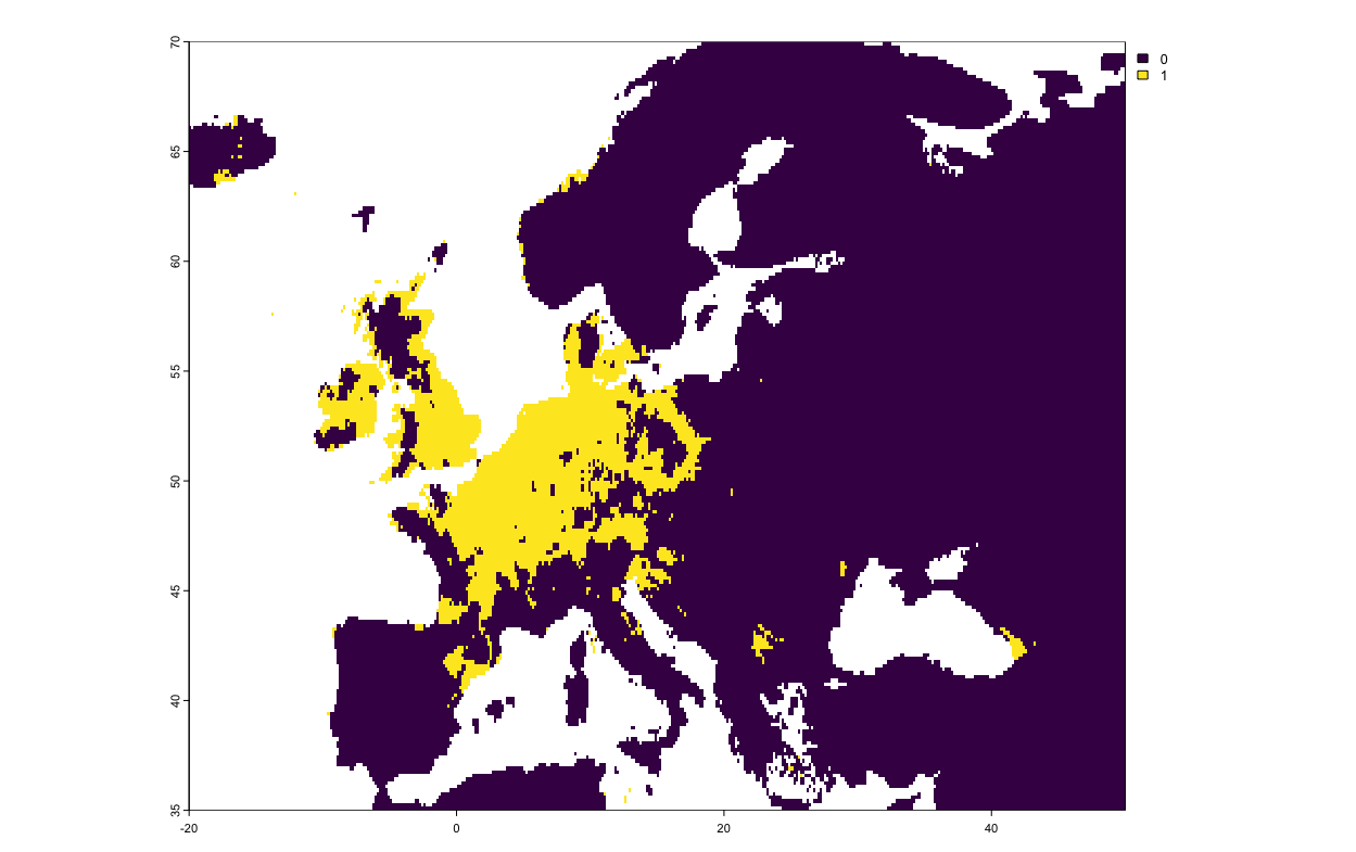
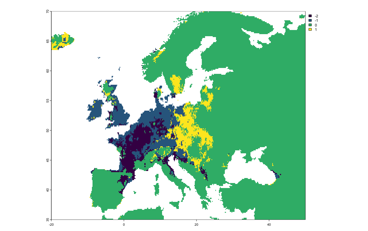
The numbers in the figure correspond to:
-2: Predicted to be lost.
-1: Predicted to remain occupied.
0: Predicted to remain unoccupied.
1: Predicted to be gained.