Module 6: Running the Model and Interpreting Results

This module provides the R code to bring everything together. We will load the data, forecast the predictors, run the Stan model, and visualize the 10-day forecast.

This script will perform the following steps:

Load the required libraries and the synthetic data.
Prepare the data into a list format that Stan can understand, including forecasted future predictor values.
Compile and run the Stan model.
Extract the posterior predictions and calculate the cumulative risk.
Generate a plot of the 10-day cumulative forecast.

# Load libraries
library(rstan)
library(tidyverse)
library(patchwork)

# 1. Load Data
# Make sure you have run the script from Module 2 to generate this file.
all_data <- read_csv("nhs_opel_data.csv")

# Create the binary outcome variable: 1 if OPEL-4, 0 otherwise
all_data <- all_data %>%
  mutate(is_opel_4 = ifelse(opel_level == 4, 1, 0))

# 2. Prepare Data for Stan (including forecasted predictors)
# This part would typically be done in Module 3, but is included here for a complete script.
library(forecast)

admissions_ts <- ts(all_data$daily_admissions, frequency = 7)
fit_admissions <- auto.arima(admissions_ts)
forecast_admissions <- forecast(fit_admissions, h = 10)

absences_ts <- ts(all_data$staff_absences, frequency = 7)
fit_absences <- auto.arima(absences_ts)
forecast_absences <- forecast(fit_absences, h = 10)

stan_data <- list(
  N = nrow(all_data),
  y = all_data$is_opel_4,
  daily_admissions = all_data$daily_admissions,
  staff_absences = all_data$staff_absences,
  N_future = 10, # We want to predict 10 days into the future
  future_daily_admissions = as.array(forecast_admissions$mean),
  future_staff_absences = as.array(forecast_absences$mean)
)

# 3. Compile and Run the Stan Model
# This will compile the model written in `opel_model.stan`. 
# This step can take a few minutes the first time you run it.
fit <- stan(
  file = "opel_model.stan",  # The path to your Stan model file
  data = stan_data,
  iter = 2000, chains = 4, cores = 1 # Standard MCMC settings
)

# 4. Extract and Process Predictions for Cumulative and Daily Risk with Credible Intervals
# The `y_pred` object is a matrix where each row is a simulation
# and each column is a day in the future (1=OPEL-4, 0=Not).
# The `p_opel_4_pred` object contains the underlying probabilities.
predictions_y <- rstan::extract(fit, pars = "y_pred")$y_pred
predictions_p <- rstan::extract(fit, pars = "p_opel_4_pred")$p_opel_4_pred

# Calculate the daily probability of OPEL-4 (median and 95% CI)
daily_prob_summary <- apply(predictions_p, 2, function(x) c(median = median(x), quantile(x, c(0.025, 0.975)))) %>%
  t() %>%
  as_tibble() %>%
  rename(median = `median`, lower = `2.5%`, upper = `97.5%`)

# 5. Visualize the Forecast (Cumulative Line with Daily Points and Credible Intervals)
forecast_df <- tibble(
  day = 1:10,
  daily_median = daily_prob_summary$median,
  daily_lower = daily_prob_summary$lower,
  daily_upper = daily_prob_summary$upper
)

ggplot(forecast_df, aes(x = day)) +
  # Daily Probability with Credible Interval
  geom_ribbon(aes(ymin = daily_lower, ymax = daily_upper), fill = "gray", col="black",alpha=0.25) +
  geom_line(aes(y = daily_median), color = "#DC241F", linewidth = 1) +
  
  scale_y_continuous(labels = scales::percent, limits = c(0, 1)) +
  scale_x_continuous(breaks = 1:10) +
  labs(
    title = "10-Day Forecast: Daily Probability of OPEL-4",
    subtitle = "Red line/ribbon: Daily Probability (median and 95% CI).",
    x = "Days from Today",
    y = "Probability"
  ) +
  theme_minimal(base_size = 14)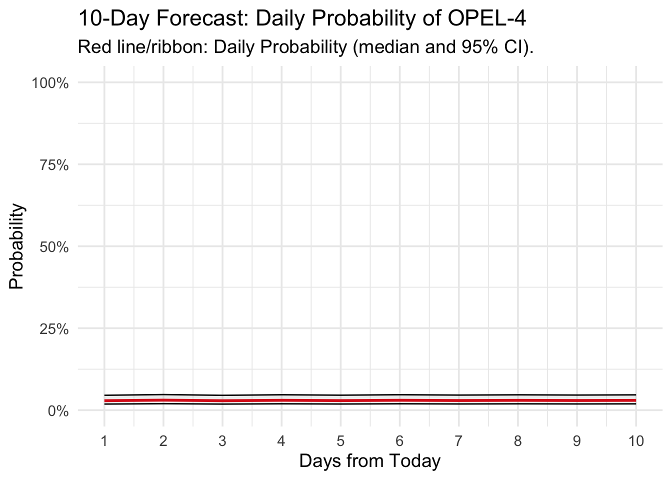

2. Interpreting the Output

When you run the stan() function, you will see a lot of output in the console as the model compiles and runs. This is normal.

Once it’s finished, you can inspect the fit object by running print(fit). This will show you a summary of the posterior distributions for all the parameters (alpha, beta_admissions, beta_absences). You can use this to see the estimated effect of each predictor.

3. The Final Visualization

The ggplot code at the end produces the key output of this entire project: a cumulative risk plot. This is a clean, easy-to-understand chart showing the total probability of the system entering OPEL-4 at least once within the next 1, 2, 3… up to 10 days.

This is the kind of actionable intelligence that can help hospital managers make proactive decisions. For example, if the plot shows that there is a 60% chance of an OPEL-4 event occurring sometime in the next 7 days, managers could schedule additional staff or free up beds in anticipation. This is often more useful than knowing the probability for a single day.

Congratulations! You have successfully built and run a Bayesian forecasting model.

← Module 5: Building the Model

Module 7: Next Steps →